Test cases
We will provide input and geometry files for all relevant test cases. These test cases will be part of the submission system.
Note
The test cases here should be a safe baseline for developing your code. Please play around with different coupling strategies and the parameters controlling preCICE. Study how the parameters affect the simulation (number of coupling iterations, solution etc.) and when the coupling gets unstable.
Note
17 Dec 2019: The remaining test cases have been updated.
13 Dec 2019: The first test case has been updated.
07 Jan 2020: Fixed error in solid solver input files (readDataName/writeDataName where swapped) and added additional results for debugging.
Forced convection over a heated plate
We have a rectangular geometry for the channel. The fluid enters the domain from the due to a pressure gradient of \(\delta p = 0.005\). The Reynolds number is \(\mathrm{Re}=500\) and the Prandtl number is \(\mathrm{Pr}=0.01\). Gravity and volumetric expansion coefficient are set to zero.
The solid is heated from below such that its bottom temperature is fixed at \(T_{\mathrm{solid,bottom}}=0\). Its heat diffusivity is set to \(\alpha = 0.2\) and so is its initial temperature.
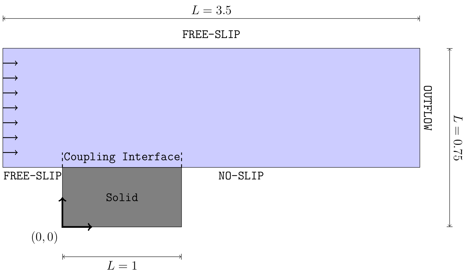
Fig. 17 Sketch of the domain of the forced convection over a heated plate.
Explicit coupling
You can find the detailed setting in the zip-file. The zip-file also contains some helper scripts (Allrun.sh and Allclean) that will run both solvers (must be in same directory) and remove all simulation results. A precice-configuration for explicit coupling is included
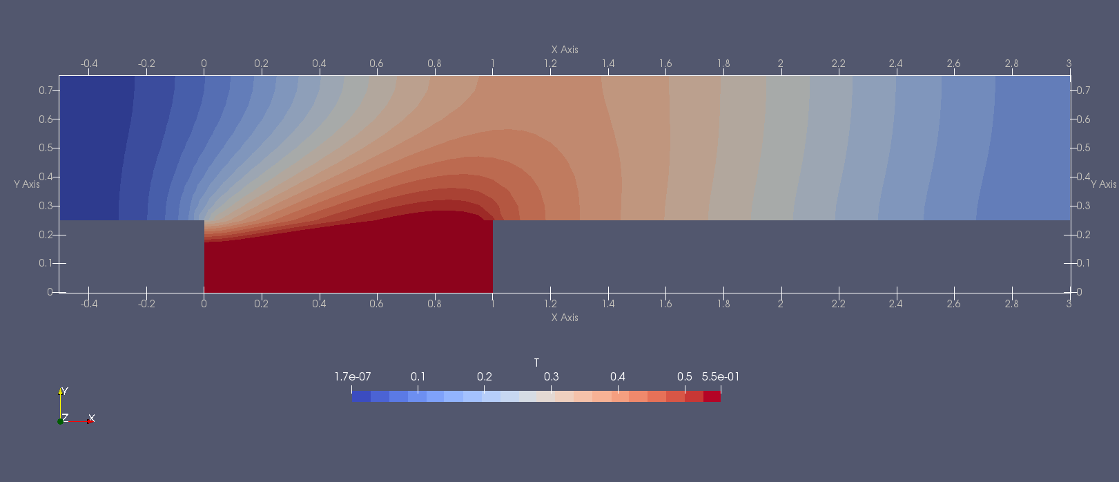
Fig. 18 Solution obtained with the input files below.
Debugging
In order to help with debugging you can find a few time steps with debugging output here: Download files.
Implicit coupling
The test case in the given configuration works with the explicit coupling scheme. You can also try to run it with an implicit coupling scheme.
Natural convection in a cavity with heat-conducting walls
The second test case is similar to the natural convection test cases from the precious exercise sheet. This time the fluid domain is not heat directly, but it is surrounded by a solid enclosure which is heated on the left and cooled on the right.
You can find the problem setup below:
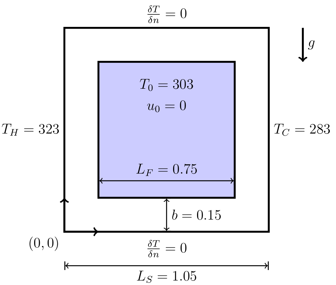
Fig. 19 The setup of the natural convection test case. The fluid domain is marked blue and the solid domain is marked in white.
The initial temperature of the solid is set to \(T_{\mathrm{solid,init}}=303\) and the heat diffusivity of the solid is \(\alpha_{\mathrm{solid}}=1\). We set the fluid the initial temperature is set to \(T_{\mathrm{fluid,init}}=303\). Prandtl number and Reynolds number are set to \(\mathrm{Pr} = 0.01\) and \(\mathrm{Re}=1000\). Additionally, we enable gravity \(\vec{g}=(0, -9.81)^T\) and the volumetric expansion coefficient \(\beta = 0.2\).
Below you can find the sample solution at different times:
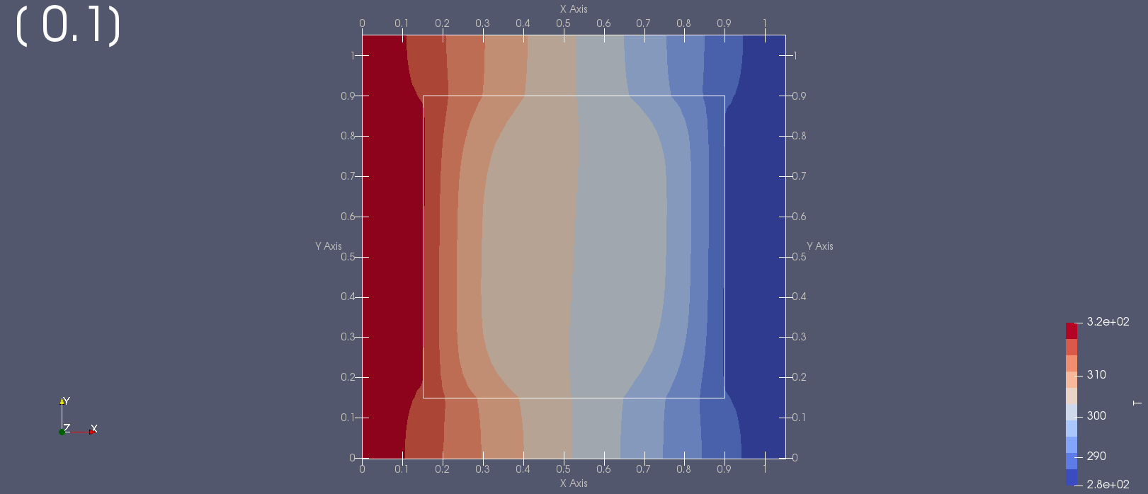
Fig. 20 Solution obtained at \(t=0.1\).
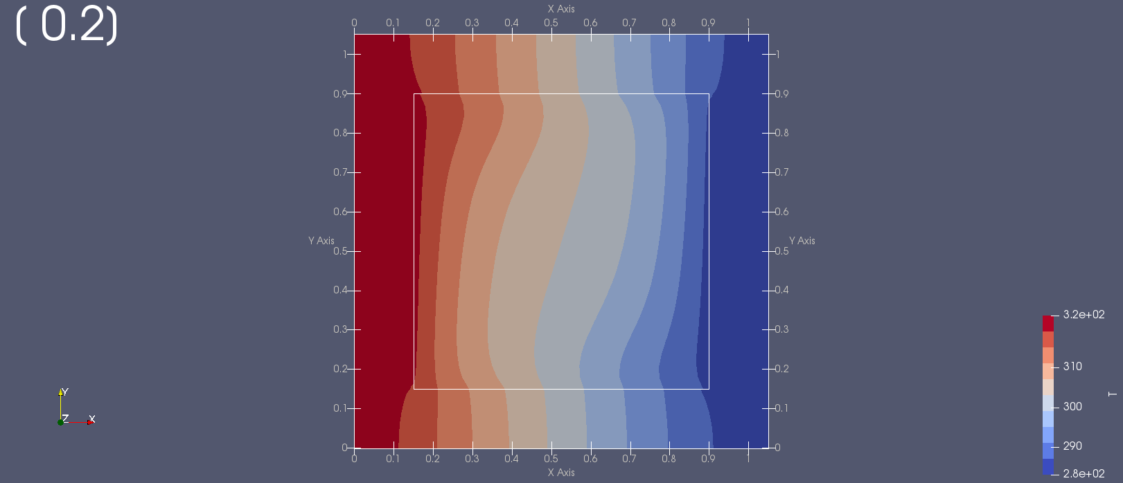
Fig. 21 Solution obtained at \(t=0.2\).
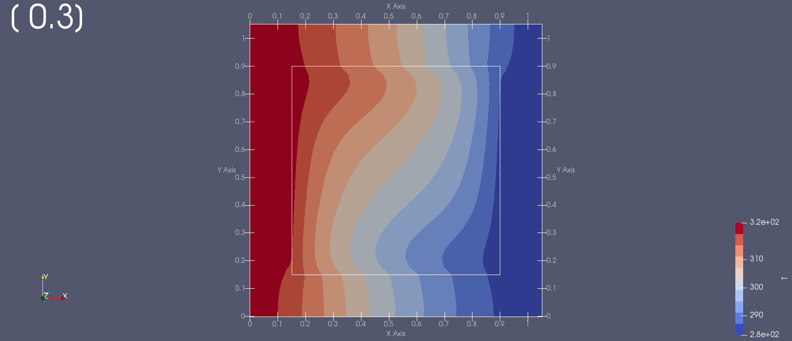
Fig. 22 Solution obtained at \(t=0.3\).
One can observe how the flow inside the fluid domain starts twisting the temperature field. The interface separating the solid domain and the fluid domain is indicated by the white line inside the domain. The solid solver marks the inner part of its domain as “inner obstacles” such that no solution is computed here. Therefore, a lot of values of the solution are set to nan there:
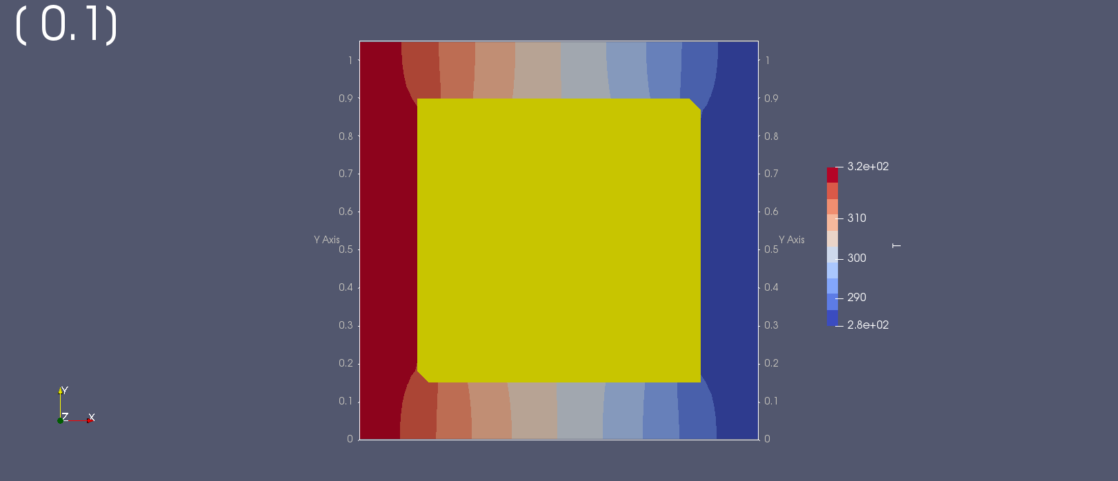
Fig. 23 The simulation domain of the solid solver.
Implicit coupling
You can find the files used to compute the solution presented above in the zip-file. Note that the parameter endTime in the input files is set to \(10\)! The time loop of the simulation should be controlled by preCICE such that the simulation actually ends for \(t<10\).
Play around with the parameters (coupling scheme, time step size etc.)! See how the solution develops for larger simulation times (max-time in the preCICE-configuration file).
Debugging
In order to help with debugging you can find a few time steps with debugging output here: Download files.
Explicit coupling
You can use the provided files to set up an explicit coupling scheme. Does it work?
2D heat exchanger (optional)
A heat exchanger is a tool that heats up a cold target fluid (here fluid domain 2) by a warm fluid (here fluid domain 1) without mixing both fluids. The two fluid domains, see figure below, are aligned at the four thin gray bars. The four bars are the solid participant. Depending on your implementation, you may need to adjust the geometry files. Experiment with different shapes, parameters and ‘turning on’ gravity, to allow for a better exchange of heat.
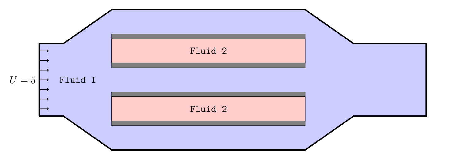
Fig. 24 Domain of fluid 1.
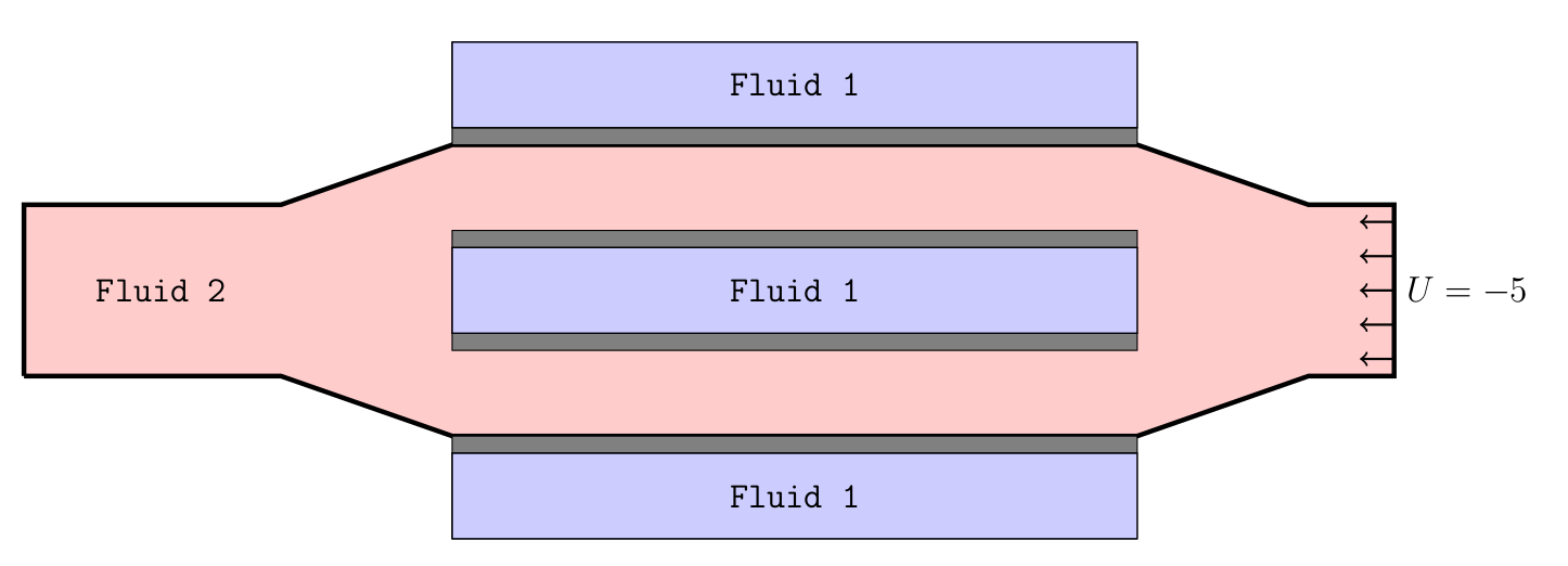
Fig. 25 Domain of fluid 2.
Note
It is optional to run the test case.
If you want to run this test case and need help with setting up the domain and configuration files, please get in touch with us.