Preparing the Solid Solver
We will derive a solid solver from the flow solver that you have implemented. The idea is that you reuse the flow solver, but fix the velocities to be zero at all times. You can do so by removing/commenting out all functions that are used for computing velocities. This means that you do not need to compute \(F\), \(G\), \(p\) and so on. The time step restrictions due to convective terms should not play a role for the time-stepping.
The solid solver should solve implicitly for the temperature. Reuse the implementation of the Gauss-Seidel scheme that you have implemented already for solving the heat equation.
Adapt your CMake-files such that an additional executable numsim_solid is build.
Gauss-Seidel/SOR solver
Reuse the implementation that you have already used for the pressure solver. Note that the grid width \(\Delta x\) and \(\Delta y\) can be different values. In the lecture they were assumed to be identical.
You need to solve the following Poisson-like equation:
In the test cases studied we do not have any heat source \(Q\).
Note
There might have been a type in the lecture notes when the Poisson-like equation was introduced. The equation above should be correct.
Input files
The geometry and input files follow the same format as the fluid solver and are only adapted slight. An example of the files can be found in the zip-file available in Section Running code without preCICE.
Geometry file
The geometry file follows the same format as for the fluid solver. We will not change anything here so you can reuse the file parser of the fluid solver. In order to make life easier we will do the follwing for geometries in the solid solver:
There will not be any solids/obstacles inside the domain. You still need obstacles in the fluid solver if you want to solve the optional test case.
The inner of the domain where heat is transported will be marked with
Feven though the solid solver models heat transport in a solid. We will use theSmarker still for parts of the domain where no computations should be carried out. This will be explained in more detail in Extension for Natural Convection Test Case.On the boundaries, we will still specify string that indicate a velocity boundary condition. You can safely ignore that. Keeping it in the geometry file should make it easier for you to reuse your file parser from the fluid solver.
Parameter file
We will use the following additional parameters:
heatDiffusivity: This is \(\alpha = \frac{\kappa}{\rho c_p}\). This is not the \(\alpha\) from the Donor-cell scheme that is used in the fluid solver. Compute the heat flux as \(q = - \alpha \frac{\partial T}{\partial n}\). For simplicity we assume that \(\rho c_p=1\) here.temperatureSolver: Can be either set toSORorGaussSeidel. If you do only implement one of the two solvers, you may ignore the parameter.omega: Relaxation factor for SOR-method. If you have not implemented the SOR-method, you may ignore it.maximumDt: Maximum time step size. It can still be smaller since preCICE might change it.
The following parameters have the same meaning as for the fluid solver:
geometryFileendTimeparticipantName: Also here the output directory should beout_${participantName}. So if one setsparticipantName=solidthe output directory should beout_solid.meshNamepreciceConfigFilereadDataNamewriteDataNametInitoutputFileEveryDtepsilonmaximumNumberOfIterations
An example input file could look like this:
# Settings file for numsim program
# Run ./numsim driven_cavity.txt

# Problem description
geometryFile = heatedbar_20x20.geom
endTime = 20.0        # duration of the simulation
participantName = NumSimSolid
meshName = NumSimSolidMesh
preciceConfigFile = precice-config.xml
readDataName = Heat-Flux
writeDataName = Temperature

heatDiffusivity = 0.01

tInit = 0

# Discretization parameters
maximumDt = 1.0       # maximum values for time step width

# Solver parameters
temperatureSolver = SOR
omega = 1.5
epsilon = 1e-5        # tolerance for 2-norm of residual
maximumNumberOfIterations = 1e4    # maximum number of iterations in the solver

outputFileEveryDt = 0.5
CMakeFile
It is easiest to add another project to the CMakeLists.txt that you have already in your src/ directory. You can copy and paste more or less everything that you have in the file for the fluid solver already. Make sure that you add all the cpp-files that you need for the solid solver to your CMakeLists.txt. Make sure that you have an executable called numsim_solid after building your solid solver!
The CMakeLists.txt for the sample solution looks similar to this (shortened version):
project(numsim_fluid)

# Things needed for the fluid solver
# ...

# install numsim_fluid executable in build directory
install(TARGETS ${PROJECT_NAME} RUNTIME DESTINATION ${PROJECT_SOURCE_DIR}/../build)

project(numsim_solid)

add_executable(${PROJECT_NAME}
   numsimsolid.cpp
   output_writer/output_writer.cpp
   output_writer/solidoutputwriterparaview.cpp
   output_writer/solidoutputwritertext.cpp
   # ...
   # and so on. Add your own files needed here!
   )
target_include_directories(${PROJECT_NAME} PUBLIC ${PROJECT_SOURCE_DIR})

find_package(VTK)

#add_executable(vtk_test vtk_test.cpp)
if (VTK_FOUND)
  include_directories(${VTK_INCLUDE_DIRS})
  target_link_libraries(${PROJECT_NAME} PRIVATE ${VTK_LIBRARIES})
endif(VTK_FOUND)

find_package(precice REQUIRED CONFIG)
target_link_libraries(${PROJECT_NAME} PRIVATE precice::precice)

add_compile_options(-Wall -Wextra)

option(STRICT "Treat warnings as errors." ON)
if(STRICT)
  add_compile_options(-Werror)
endif()

message("If VTK was found on the system: VTK_FOUND: ${VTK_FOUND}")
message("The directory of VTK: VTK_DIR: ${VTK_DIR}")
message("The include directory of VTK: VTK_INCLUDE_DIRS: ${VTK_INCLUDE_DIRS}")
message("The directory of preCICE: precice_DIR: ${precice_DIR}")
message("CMAKE_BUILD_TYPE: ${CMAKE_BUILD_TYPE}")
message("PROFILE: ${PROFILE}")

# install numsim_solid executable in build directory
install(TARGETS ${PROJECT_NAME} RUNTIME DESTINATION ${PROJECT_SOURCE_DIR}/../build)
Running code without preCICE
If you want to test your code, it can be useful to run alone with out a second solver. However, if you have preCICE integrated, it will always wait for (at least) a second participant.
You can avoid that by defining a new option in your CMakeLists.txt. You could for example add the option WITHPRECICE that is on by default. It will set a definition called WITHPRECICE that you can check for in your code.
option(WITHPRECICE "Compile with preCICE activated." ON)

if(WITHPRECICE)
  # Add preCICE to project
  add_definitions(-DWITHPRECICE)
endif()
You can then use the definition in your code like this:
#ifdef WITHPRECICE
  //Do preCICE calls here
  SolverInterface interface(configName, 0, 1);
#else
  //Things to do if it is not a preCICE run
#endif
The submission that you upload must be using preCICE by default! We do not check for any extra option that you define in your configuration.
Verification
We would suggest to test your implementation by setting up a test case with insulating walls at opposite side. The other two sides should have fixed temperatures. After sufficient simulation time you should see a linear temperature profile.
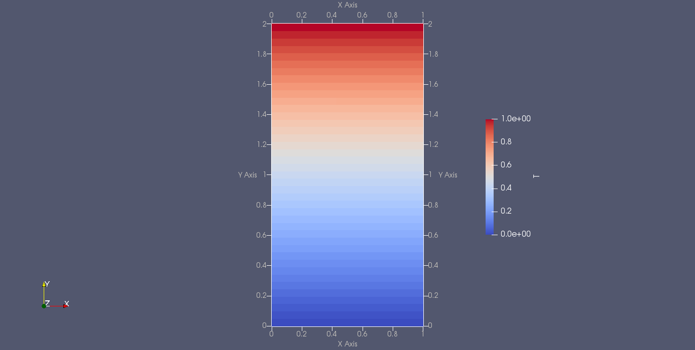
Fig. 14 Solution of the heat equation for a vertical bar. The top is heated \(T_{\mathrm{top}}=1\) while the bottom is cooled \(T_{\mathrm{bottom}}=0\).
The simulation results and an input file (that does not use preCICE) can be found here: Download files.
Extension for Natural Convection Test Case
You will need to have boundary conditions inside the domain. Make sure that your code can handle this. The boundaries are currently marked as NSW;TPD such that you can reuse your input file parser. Please check Natural convection in a cavity with heat-conducting walls for an example how the geometry file looks like.
You have to take care of the corners. At these points the solid solver is coupled to the fluid solver at two different sides. For example, the situation of the top left corner of the fluid solver should be like

Fig. 15 The top left corner of the fluid solver is surrounded by coupling cells.
The coupling (ghost) cells used for boundary conditions are marked in green (C).
The solid solver sees the opposite situation

Fig. 16 The top left corner of the fluid solver seen from the solid solver. One has two coupling counditions in the center cell since there is a coupling between the vertical and the horizontal face.
Tasks
Write a solid solver for the heat transport equation .
Extend your code such that it can have boundary conditions inside the domain. This will be needed in the natural convection test case.