Tasks

To get started with PyTorch, we will build and test our project in four steps:

First, we will set up the training pipeline as explained in the tutorial and overfit the network from a randomized input image to some specific image like the SGS logo (see below). This confirms that the training loop and the model setup work correctly and that the dimensions fit.

Second, we will overfit the model to a single simulation output. This requires data generation and preparation, described in detail below. This initial test should result in a very small remaining error and no systematic errors. If this works, we know that our data preparation - including appropriate normalization - is correct and that there are no underlying issues preventing the network from learning this output. Since we overfit to only one data point, the network does not yet need to learn to distinguish between different output scenarios.

Hence, the third test consists of overfitting to ten simulation outputs. This allows us to verify that the inputs contain enough information for the network to differentiate between different simulations and that no additional inputs are needed.

The final step is to train on the full dataset. Introduce splitting into training, validation, and test subsets. Check that both the training and validation losses decrease over time to avoid overfitting.

Data Generation

To generate a dataset for training, we need variation in the inputs. In this exercise, we vary the Reynolds number and the boundary condition of u simultaneously. The minimum Reynolds number is 500 with dirichletTopX = 0.5; the maximum values are Re=1500 and dirichletTopX = 1.50. We used equally spaced values. All other parameters are the same as in exercise 1 (lid-driven cavity) in this folder.

The final simulation time is 10 seconds.

We want 101 data points (simulations) for training the neural network.

Follow the first steps of the tutorial Lid-driven cavity and modify the configuration files to match our previous default simulation scenario.

Data Preparation

Since the variations in Re and in the boundary condition of u are directly connected, we only need one of them as the network input.

To reduce the inputs to the bare minimum, we handcraft a single channel of initial boundary conditions of size (1, len(output field), width(output field)), initially filled with zeros. Then inputs[0, -1, 1:-1] = ux-value.

For the labels, we extract the u and v fields at the last timestep and form one data point of size (2, len(output field), width(output field)) as in Fig. 13.

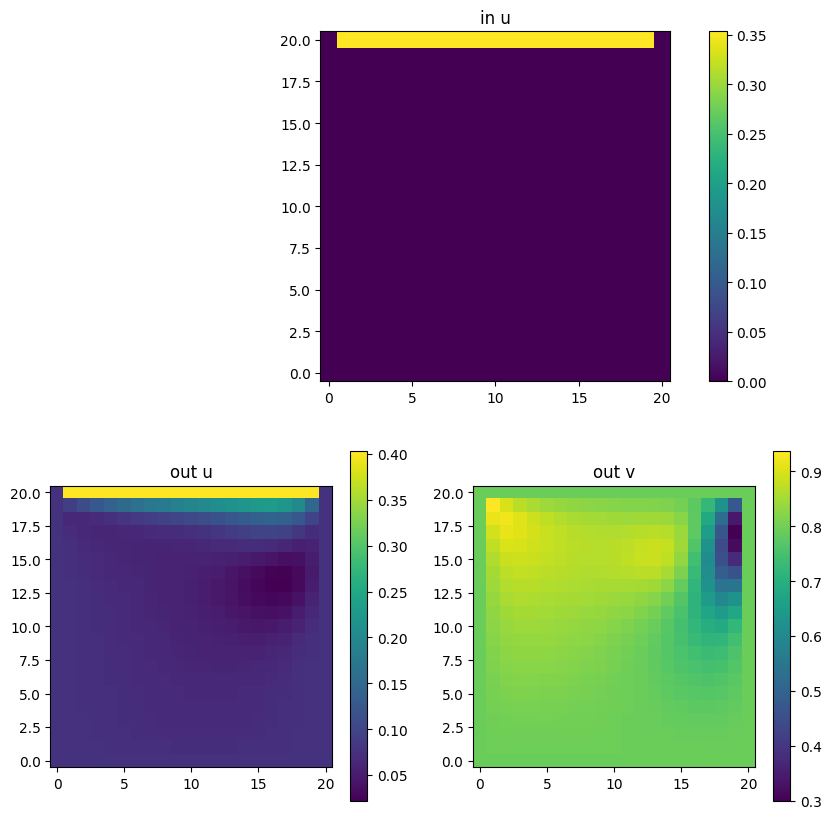
../_images/example_inputs_labels.png — Fig. 13 Example data point with handcrafted input and the two output fields u and v.

All data points are concatenated along the first axis, yielding a dataset of shape data points × channels × field length × field width for both inputs and labels.

Each channel must be normalized separately to the range (0, 1) via rescaling. Store the original minimum and maximum values per channel in a min_max.yaml file so you can later reverse the normalization for visualizations and evaluation. The file should look like this:

inputs:
u:
        max: # maximum u-value (provided as input to the simulation as an initial condition)
        min: # minimum u-value (provided as input to the simulation as an initial condition)
labels:
u:
        max: # maximum found value for u
        min:  # minimum found value for u
v:
        max:  # maximum found value for v
        min:  # minimum found value for v

The prepared dataset can either be stored in memory or kept in cache.

For real training (not the overfitting tests), remember to shuffle and split the samples into training (80%), validation (10%), and test (10%) sets.

Model Setup and Training Parameters

The reference model is a CNN with the following layers:

Conv2d(in=1, out=16, kernel=7x7, padding=”same”, stride=1 (other hyper-params default)
ReLU
five hidden layers, each consisting of:
- Conv2d(in=out=16, rest same as before)
- ReLU
final layer: Conv2d(in=16, out=2, rest same as before)

Training parameters:

learning rate: 1e-3
epochs: 4000
optimizer: Adam
loss function: MSE

Note

Feel free to adjust the architecture, but keep the model size below 1 MB (check via path -ll …). You can also experiment with training parameters, separate the two outputs into independent models, add learning-rate scheduling, use different optimizers or losses, investigate different weight initializations, or try architecture variants (e.g., fully connected networks, NeRF-like networks, or pure CNN decoders - for those we also have sample solutions). If you change the loss function, keep the final comparison metric the same (e.g., validation loss) so that models remain comparable.

Storing your Model

Once you’re done training you can store your model via

model_path = f"{model_name}.pt"
torch.save(model.state_dict(), model_path)

To check that it worked, you can load it by

# initializing an empty model
model = init_my_model()

# loading your stored model
model.load_state_dict(torch.load(model_path))
model.eval()

Applying your Model to New Data

Load and prepare data as before, but do not perform a train/val/test split. Do not rescale using new min/max values—use the min/max values stored in min_max.yaml that come with the model. Set the model to evaluation mode: model.eval().

Model Evaluation

Qualitative analysis: Plot training and validation loss in one figure. Plot exemplary predictions of u and v and compare them to the ground truth via absolute difference. (Optionally: visualize the velocity field via plt.quiver(u_field, v_field). Remember to rescale the data back to the original ranges beforehand.)

Quantitative analysis: Compute RMSE and MAE per channel in the original (un-normalized) units.

Out-of-distribution (OOD) evaluation: These tests check whether the model generalizes beyond what it has seen during training. Apply your model to three out-of-distribution cases as described below and hand-in the results. We will discuss them during the oral exam. Make sure to only change one thing at a time (while the rest of the parameters is the same as in the training data) for a clear analysis.

Different Reynolds numbers (same geometry): Re and u values: set Re=3000 and u accordingly.

Larger spatial domain: Keep Re and u in-distribution but change the spatial domain from 21x21 cells to 41x41 cells - same cell-width but larger physical field.

Different boundary conditions: Put the passing-by-flow-BC to the left instead of the top.

Leaderboard on Kaggle

To evaluate how well your model performs, please upload it as a submission to kaggle whenever you want and as often as you like: https://www.kaggle.com/t/749e05c9967b4d46bd9cb929dce962b2.

There you can compare your results with other groups and with our sample solution.

Instructions for making a submission are available on the competition page (a Kaggle account is required but easily generated).